NSE:: National Stock Exchange of India Limited is one of the
leading Stock Exchange in India, based in Mumbai. NSE is under the ownership of
various financial institutions such as banks and insurances.
It’s the world’s largest derivatives exchange by number of contracts
traded and the third largest in cash equities by number of trades for year
2022. It is one of the largest stock exchanges in the world by market
capitalization.
Requirements: Microsoft Excel 2016 or later version
Lit bit knowledge of HTML, IE to find Cookies and links
Lit bit knowledge of Excel & Macros.
Rest you leave on this post 😊 just follow all steps carefully and don’t miss anything.
Step 1: Go to NSE Website
(https://www.nseindia.com) then go to Derivatives
à Options à Nifty50 à Option Chain then right click on webpage.
Then
Copy Cookie and Goto Excel.
Step 2: Make 3 Sheets in Excel Workbook. Name: Cookies,
Nifty50, Source.
Step 3: In Cookies Sheet, Name Cell A2 as Cookies and Paste Cookie in A3 cell.
Step 4: Go to Sheet Source, then click on Data Tab then Goto New Query à From Other Source à Blank Query.
Step 5: Rename it with ExpiryDate. Then right click on query à Advance Editor, Clear the values showing there and paste as I mentioned below.
let
Source =
Json.Document(Web.Contents("https://www.nseindia.com/api/option-chain-indices?symbol=NIFTY",
[Headers=[Referer="https://www.nseindia.com/get-quotes/derivatives?symbol=NIFTY",
#"User-Agent"="Mozilla/4.0 (compatible;MSIE6.0; Windows
NT5.1", Accept="text/html; charset=utf-8",
#"Accept-Language"="en-us,en;q=0.9", #"Accept-Encoding"="gzip,deflate",
Cookie="Cookie copied from website"]])),
records =
Source[records],
expiryDates =
records[expiryDates],
#"Converted to Table" = Table.FromList(expiryDates,
Splitter.SplitByNothing(), null, null, ExtraValues.Error),
#"Renamed
Columns" = Table.RenameColumns(#"Converted to
Table",{{"Column1", "Expiry"}})
in
#"Renamed
Columns"
Step 6: Close and Load to Cell D3 of sheet “Source”.
Step 7: Repeat step 4 and 5, rename query with StrikePrice then
Close & load to Cell A3 of Sheet “Source”
let
Source =
Json.Document(Web.Contents("https://www.nseindia.com/api/option-chain-indices?symbol=NIFTY",
[Headers=[Referer="https://www.nseindia.com/get-quotes/derivatives?symbol=NIFTY",
#"User-Agent"="Mozilla/4.0 (compatible;MSIE6.0; Windows
NT5.1", Accept="text/html; charset=utf-8",
#"Accept-Language"="en-us,en;q=0.9",
#"Accept-Encoding"="gzip,deflate", Cookie="Cookie"]])),
records =
Source[records],
#"Converted to Table" = Record.ToTable(records),
#"Filtered
Rows" = Table.SelectRows(#"Converted to Table", each ([Name] =
"timestamp" or [Name] = "underlyingValue")),
#"Transposed Table" = Table.Transpose(#"Filtered
Rows"),
#"Promoted
Headers" = Table.PromoteHeaders(#"Transposed Table",
[PromoteAllScalars=true]),
#"Changed
Type" = Table.TransformColumnTypes(#"Promoted
Headers",{{"timestamp", type datetime},
{"underlyingValue", type number}}),
#"Renamed
Columns" = Table.RenameColumns(#"Changed
Type",{{"timestamp", "TimeStamp"},
{"underlyingValue", "StrikePrice"}})
in
#"Renamed
Columns"
Step 8: Repeat Step 4
and 5, rename query with Nifty50 then close & load to Cell F3 of sheet “Source”
let
Source =
Json.Document(Web.Contents("https://www.nseindia.com/api/option-chain-indices?symbol=NIFTY",
[Headers=[#"Accept-Encoding"="gzip, deflate",
#"Accept-Language"="en-US,en",
#"User-Agent"="Mozilla/5.0 (Windows NT 10.0; Win64; x64)
AppleWebKit/537.36 (KHTML, like Gecko) Chrome/81.0.4044.138 Safari/537.36
OPR/68.0.3618.206", Cookie="Cookie"]])),
records =
Source[records],
data =
records[data],
#"Converted
to Table" = Table.FromList(data, Splitter.SplitByNothing(), null, null,
ExtraValues.Error),
#"Expanded
Column1" = Table.ExpandRecordColumn(#"Converted to Table",
"Column1", {"strikePrice", "expiryDate",
"CE", "PE"}, {"strikePrice",
"expiryDate", "CE", "PE"})
in
#"Expanded Column1"
Expend CE, PE with selecting “OI, OICh, IV, LTP, Change”
Till now we have completed our work almost in sheet “Cookies”
and “Source”, now we will work on main sheet named as “Nifty50”
Step: 9 In Sheet “Nifty50” we will special paste(link) values from Source sheet A4:B4 then format C4
as general.
Step 10: In Sheet “Nifty50” cell F3 à Data Validation à In source select list
of Expiry then OK.
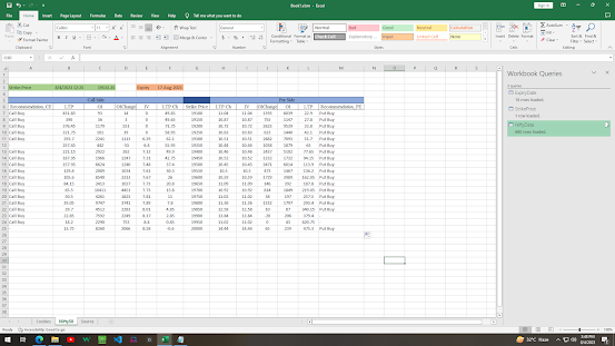
Step 11: Prepare Table format as shown in image below
(remember that keep position of table same as shown in image to avoid any
problem during paste of formula
(Note: Values and formula will be placed from cell no. 7 in
table.)
Step 12: In Cell G16 Paste formula “=MROUND(C3,50)”
Step 13: in upper cells use “=G16-50” and in lower cells use
“=G16+50”
Step 14: Copy Formula in F7
=SUMIFS(NiftyData[CE.change],NiftyData[expiryDate],Nifty50!F$3,NiftyData[strikePrice],Nifty50!G7)
Step 15: Copy Formula in E7:
=SUMIFS(NiftyData[CE.impliedVolatility],NiftyData[expiryDate],Nifty50!F$3,NiftyData[strikePrice],Nifty50!G7)
Step 16: Copy Formula in D7:
=SUMIFS(NiftyData[CE.changeinOpenInterest],NiftyData[expiryDate],Nifty50!F$3,NiftyData[strikePrice],Nifty50!G7)
Step 17: Copy Formula in C7:
=SUMIFS(NiftyData[CE.openInterest],NiftyData[expiryDate],Nifty50!F$3,NiftyData[strikePrice],Nifty50!G7)
Step 18: Copy Formula in B7:
=SUMIFS(NiftyData[CE.lastPrice],NiftyData[expiryDate],Nifty50!F$3,NiftyData[strikePrice],Nifty50!G7)
=IF(AND(D7>0,OR(F7>0)),"Call Buy","-")
Step 20: Copy Formula in H7:
=SUMIFS(NiftyData[PE.impliedVolatility],NiftyData[expiryDate],Nifty50!F$3,NiftyData[strikePrice],Nifty50!G7)
Step 21: Copy Formula in I7:
=SUMIFS(NiftyData[PE.impliedVolatility],NiftyData[expiryDate],Nifty50!F$3,NiftyData[strikePrice],Nifty50!G7)
Step 22: Copy Formula in J7:
=SUMIFS(NiftyData[PE.changeinOpenInterest],NiftyData[expiryDate],Nifty50!F$3,NiftyData[strikePrice],Nifty50!G7)
Step 23: Copy Formula in K7:
=SUMIFS(NiftyData[PE.openInterest],NiftyData[expiryDate],Nifty50!F$3,NiftyData[strikePrice],Nifty50!G7)
Step 24: Copy Formula in L7:
=SUMIFS(NiftyData[PE.lastPrice],NiftyData[expiryDate],Nifty50!F$3,NiftyData[strikePrice],Nifty50!G7)
Step 25: Copy Formula in M7:
=IF(AND(H7>0,OR(J7>0)),"Put Buy","-")
Now drag all formula to complete table as show in below
image

Step 25: by conditional formatting make it more usable like shown below
Now we will create 3 buttons and will assign macros to them.
To create Macros just copy & Paste below code:
Public t As Date
With
CreateObject("WinHttp.WinHttpRequest.5.1")
.Open "GET", URL, False
.setRequestHeader "User-Agent",
"Mozilla/4.0 (Compatible;MSIE 6.0;Windows NT 5.1)"
.setRequestHeader "Accept",
"text/html;charset=utf-8"
.setRequestHeader
"Accept-Language", "en-us,en;q=0.9"
.setRequestHeader "Accept-Encoding",
"gzip,deflate"
.send
strCookie = .getAllResponseHeaders
strCookie = Split(strCookie, vbCrLf)
CookieN = Trim(Split(Split(strCookie(5),
";")(0), ":")(1)) & "," &
Trim(Split(Split(strCookie(6), ";")(0), ":")(1))
End With
End Function
Sub Nifty50()
Dim C As String
C =
(CookieN("https://www.nseindia.com/get-quotes/derivatives?symbol=NIFTY"))
ThisWorkbook.Sheets("Cookies").Range("A3").Value
= C
End Sub
Sub GetData()
Call Nifty50
ThisWorkbook.RefreshAll
End Sub
Sub Ref()
Call GetData
t = Now +
TimeValue("00:01:00")
Application.OnTime t,
"Ref", Schedule:=True
End Sub
Sub Stp()
On Error Resume Next
Application.OnTime t,
"Ref", Schedule:=False
End Sub
Final Result:
Thanks😊


No comments:
Post a Comment